Course Review - Causal Inference

This semester, I had the pleasure of taking a course on Causal Inference with Professor Elias Bareinboim, one of Judea Pearl’s former students and author of some seminal results in Causal Inference. I feel like this course highlighted not only the content Causal Inference researchers consider important but also the types of understanding they value. In this review, I’ll focus on the latter. I hope to write some blog posts in the future about the former but have learned from past experience not to promise future posts unless I have time during which I know I can write them.

Brief Course Content Overview #

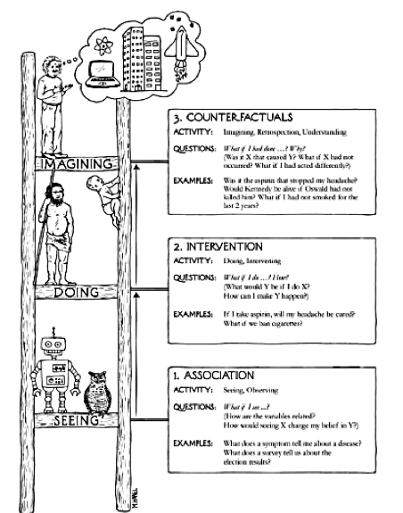
The course was organized along the rungs of the ladder of causation. As depicted below, the first rung of the ladder is association. Since many of the students, including myself, taking this course have a background in machine learning, we didn’t spend much time on this rung. We reviewed some of the results from the probabilistic graphical models literature and then recast them from a causal perspective. I’ll talk more about what this recasting looks like in the next section. The second rung of the ladder is intervention. This is about understanding how feasible manipulation of variables impacts overall systems. The bulk of our time in the course was spent on this rung. Specifically, we spent a lot of time talking about and going over the key results for identifying interventional quantities (\( \text{do}(\cdot) \) probabilities. After that, we spent some time diving into more recent results such as the stochastic calculus and causal reinforcement learning (also see this talk) that leverage and extend these results. From there, we broadened our focus to what Elias calls the “Data Fusion” problem, which is broadly about solving the problem of answering questions across the rungs. Finally, we jumped up to the third rung, counterfactuals, which is often analogized to imagination and retrospection. That is, answering the question “what would have happened if …?”

Themes #

It all starts with an SCM #

When I first encountered causality outside of the course, it was often described 1) as an extension to probabilistic graphical models or 2) as something we could use with linear relationships. This first presentation made things confusing because it was never clear which results only applied to probabilistic graphical models versus also to causal graphical models (or vice versa). The second presentation made things confusing by conflating statistical and causal language and questions. While the core results for both probabilistic graphical models and linear causal models do predate the non-parametric results in causal inference, in my humble opinion, teaching things in the historical order the wrong way to introduce causality to most people.

Thankfully, this is also not how Elias’s course introduces it. Elias does things the “right” way by starting with the structural causal model (SCM) and using it to derive non-parametric results for figuring out causal effects. I call this the right way because I think it’s conceptually much clearer in terms of starting with the most fundamental concept and then showing how everything else follows naturally from it.

Briefly, the key assumption behind structural causal models is that reality’s underlying mechanisms can be described in terms of deterministic functional relationships between observed and unobserved entities with all of the randomness coming from the unobservables. While I spent a non-trivial amount of time pestering Elias and the TAs about how ontologically this isn’t true, it’s very similar to the sorts of assumptions we make in machine learning, statistics, much of physics and chemistry, and our everyday lives, so I think it’s quite reasonable. (1) (1)Almost all of the current results in causal inference assume acyclic structural causal models, i.e. ( X ) and ( Y ) can’t both depend on each other, this is because assuming this allows us to derive more useful results, not because SCMs are inherently acyclic.

Fertilizer SCM Example #

Suppose we are modeling the effect of two fertilizers on tree growth. An over-simplified SCM for this situation would likely include two observed variables, \( F \in \{0, 1\} \) representing the two fertilizers and \( T \in \mathbb{R} \) representing the tree’s height at some pre-determined point in time after adding the fertilizer to the tree’s soil. However, we also need to account for the fact that the tree’s growth depends on myriad other factors besides the fertilizer choice – weather, soil, genetics, and presumably other factors of which I’m not aware. If we were actually modeling this situation, we’d probably measure and “control for” (2) (2)Controlling for a variable is a term from statistics that roughly means to try and understand what the relationship between the input and output variables we care about is assuming we hold the control variables constant. The image I typically have in mind when I think of controlling for variables is wiggling the input variable of interest while fixing the control variables. some of these variables, but for the sake of keeping this example simple, let’s assume we can’t measure any of them. Instead, we can decide that we’re just going to assume that these variables can all be summarized with a random variable $ U_T $.

Now, recall that I said the key assumption behind SCMs is that we can model reality with functions of observed and unobserved variables. Let’s try and do that here. Assuming the fertilizer application is done randomly (say by the flip of a coin), there’s no mechanism by which these unobserved factors can affect it, so the functions that determines fertilizer will not contain $ U_T $ as a term and instead will just be $ f_X(U_X) = U_X $ where $ U_X \sim \text{Bern}(1 / 2) $. Tree growth on the other hand, will presumably be affected by all these unobservables. For simplicity’s sake let’s suppose it’s a linear function of the unobservables plus some constant times whether we use fertilizer, $$ T \leftarrow f_T(U_T, X) = U_T + \beta X. $$ Finally, let’s suppose that we can model our unobservables as normally distributed around some mean. (3) (3)While this may seem a little weird, it’s actually not as crazy as it may seem. If you’re familiar with regression from statistics, we can think of this as a linear model with normally distributed noise ($ U $) and make some argument about it being a reasonable approximation with large sample sizes.

It turns out that the combination of the distribution over the unobservables combined with the functional relationships also induces a graph that looks like the following.

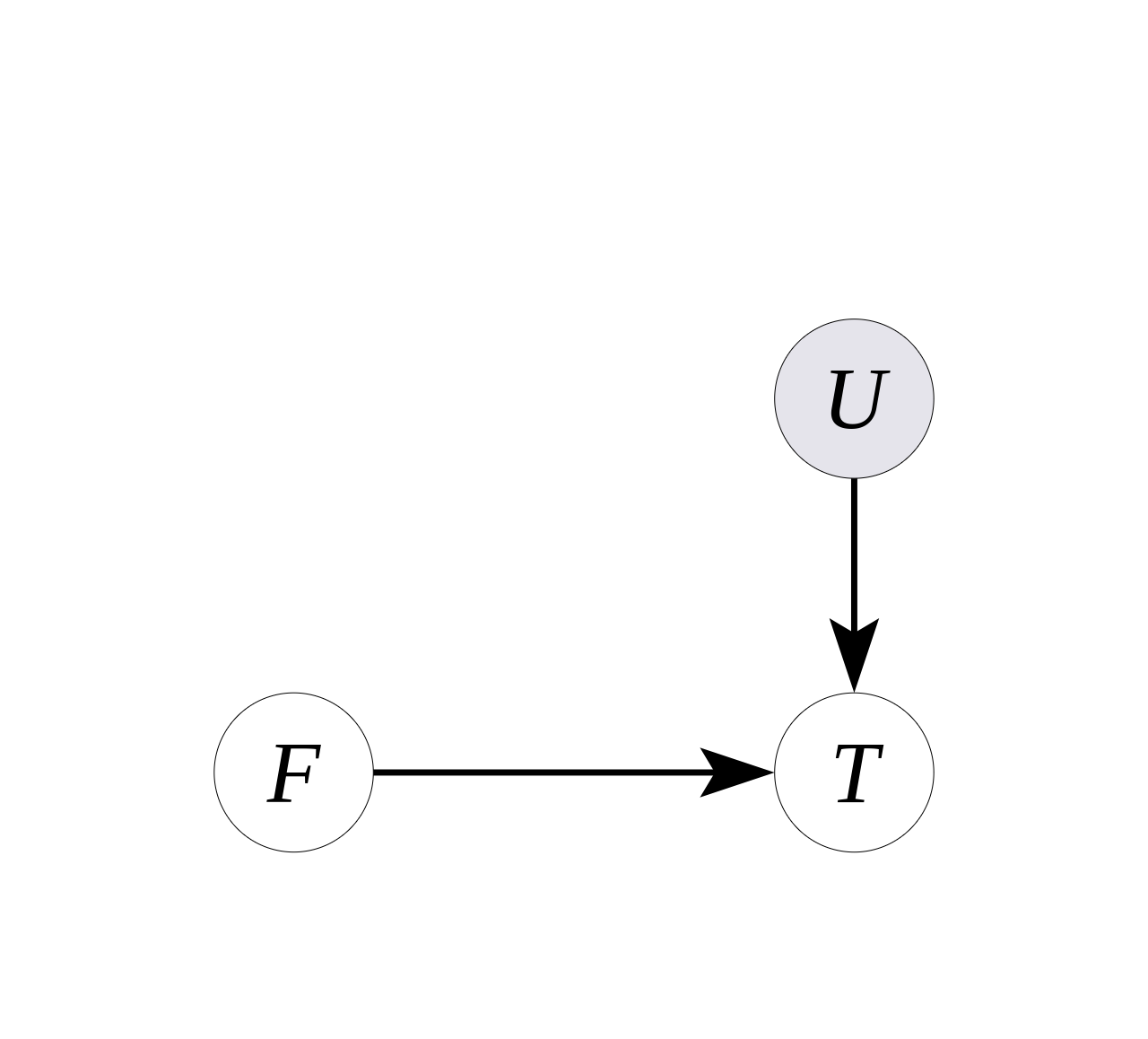
Furthermore, just by looking at the graph, we can deduce that the impact of fertilizer application on tree growth in the observed distribution is equal to the impact of intervening by adding fertilizer. This may not seem surprising because we explicitly randomized the process of fertilizer application, but where this gets interesting is that we can also obtain similar interventional quantities from observational data where it might initially seem impossible. (4) (4)For a classic example, see my post on deriving the front-door criterion. There’s lots more I could say about this, but I insetad recommend looking at other resources such as Michael Nielsen’s post, this talk by Pearl, and The Book of Why for more on the details.

Construct a counterexample #

One way to learn causal inference is to understand what it can accomplish. An alternate, in my opinion, underrated, way is to understand what it can’t accomplish. It turns out this latter form of understanding features heavily in the way Elias and his students think about and discuss the area with each other. By this I mean that for any given concept in causal inference, I suspect they could generate a few counter-examples that illuminate the core reason why the concept is non-trivial but important. This is best illustrated by example.

Simple(st) Identifiability Counterexample #

Identifiability is one of the core concepts of causal inference. Informally, identifiability is about our ability to estimate an interventional quantity given a graph and a joint distribution. In plain English, if I know the graph of how things are related and have observational data, can I estimate what value a variable (or variables) will take given that I set another (or others)? A little less informally, we say a quantity like $ P(y \mid \text{do}(x)) $ (5) (5)Probability that random variable $ Y $ takes a certain value, $ y $, given that we intervene to set $ X $ to $ x $. is identifiable if all the all models that induce the graph $ \mathcal{G} $ and joint distribution over observables $ P(\mathbf{V}) $, produce the same value for $ P(y \mid \text{do}(x)) $. To be totally honest, I’d read this definition in a bunch of different places before I took this course but didn’t really grok it because it wasn’t clear to me what wasn’t identifiable. Hopefully this counterexample is as helpful for others as it was for me.

Consider the following graph (often called the “bow graph”), in which we’ll show that $ P(y \mid \text{do}(x)) $ is identifiable.

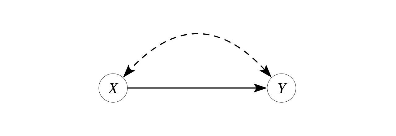
It has two binary observed variables, $ X $ and $ Y $, and one binary unobserved confounding variable $ U $. Here are two SCMs ($ \mathcal{M}_0 $, $ \mathcal{M}_1 $) that induce this same graph. $$ \begin{aligned} \mathcal{M}_0: \mathcal{F} = \{f_X, f_Y \} \text{ where } f_X(U) = U, f_Y(U, X) = (X \land U) \oplus U_Y \\\ \mathcal{M}_1: \mathcal{F} = \{f_X, f_Y \} \text{ where } f_X(U) = U, f_Y(U, X) = (X \lor U) \oplus U_Y. \end{aligned} $$ In both, $ P(U = 0) = P(U_Y = 0) = 3 / 4 $. (6) (6)A reasonable question to ask would be, “why include the $ U_Y $ variable?” The brief answer is that the definition of SCMs typically assume that all possible values of the observed variables have non-zero probability. As one can calculate for this example, this is true if we include the $ U_Y $ and false without it.

Recall, that $ P(y \mid \text{do}(x)) $ is identifiable if and only if all models that induce $ \mathcal{G} $ and have the same $ P(\mathbf{V}) $ have the same $ P(y \mid \text{do}(x)) $. Clearly these two models induce the same $ \mathcal{G} $. Let’s show they induce the same $ P(\mathbf{V}) $.

In order to compute the observed joint distribution for these two models, we can simply plug in the value of $ X $ in terms of $ U $ and get, $$ \begin{aligned} P_{\mathcal{M}_0}(X = 0, Y = 0) &= P(U = 0, U \oplus U_Y = 0) \\\ &= P(U = 0) P(U \oplus U_Y = 0 \mid U = 0) \\\ &= 3 / 16, \end{aligned} $$ and $$ \begin{aligned} P_{\mathcal{M}_1}(X = 0, Y = 0) &= P(U = 0, U \oplus U_Y = 0) \\\ &= P(U = 0) P(U \oplus U_Y = 0 \mid U = 0) \\\ &= 3 / 16. \end{aligned} $$ Both results follow from the identities $ A \land A = A \lor A = A $ and by application of the probability chain rule. If we do similar calculations for the other three possible pairs of values for $ X $ and $ Y $, we’ll find that all pairs have equal probability in both models as well. This is easy to see by noting that in both models, $ f_Y(U, X) = U \oplus U_Y $ when we substitute $ U $ for $ X $.

So both models induce the same graph and joint distribution, but what about the quantity we’re interested in, $ P(y \mid \text{do}(x)) $? To determine $ P(y \mid \text{do}(x)) $, we replace $ f_X(U) $ with the constant $ x $ everywhere $ f_X $ appears in the SCM. If we do that with our two models and intervene with $ \text{do}(X = 0) $, we get the following probabilities for $ Y = 0 $ $$ \begin{aligned} P_{\mathcal{M}_0}(Y = 0 \mid \text{do}(X = 0)) &= P((0 \land U) \oplus U_Y = 0) \\\ &= P(U_Y = 0) \\\ &= 3 / 4. \end{aligned} $$ and $$ \begin{aligned} P_{\mathcal{M}_1}(Y = 0 \mid \text{do}(X = 0)) &= P((0 \lor U) \oplus U_Y = 0) \\\ &= P(U \oplus U_Y = 0) \\\ &= P(U = 0, U_Y = 0) + P(U = 1, U_Y = 1) \\\ &= (3 / 4)(3 / 4) + (1 / 4)(1 / 4) \\\ &= 5 / 8. \end{aligned} $$ These don’t match, which means we have proven that $ P(y \mid \text{do}(x)) $ is not identifiable in graph $ \mathcal{G} $.

Having gone through all this work to show this, what was the point? In my opinion, seeing the counterexample helps one understand identifiability in a way that just learning the definition and seeing positive examples doesn’t. With respect to this specific example, this example shows how un-identifiability can arise due to effects canceling each other out in the observational distribution, even when the model’s mechanisms produce fundamentally different outcomes once we eliminate some of the randomness coming from the unobservables.

At a higher level, I think the focus on counterexamples in causal inference is relatively unique and highlights how counterexamples can play a large role in improving understanding of abstract concepts.

Show me the algorithm! #

As a computer science, programmer type, I’m very much onboard with the ‘algorithmitization’ approach to subjects. As Donald Knuth put it, “Science is knowledge which we understand so well that we can teach it to a computer.” Based on the course, causal inference researchers seem to share this view and have made impressive strides towards ‘algorithmitizing’ causal inference. For example, one of my favorite things we discussed in the course was the Identify algorithm (7) (7)Invented by Jin Tian and described in his masterpiece of a PhD thesis. Excitingly, although I haven’t yet had the chance to deeply study it, Professor Bareinboim and one of our course TAs, Juan Correa, recently extended this algorithm to a more general scenario in which additional experimental distributions, i.e. $ P(\mathbf{v} \mid \text{do}(\mathbf{z})) $, are also available for assisting with identifying the target quantity. Given a causal DAG, Identify either returns a formula for a $ \text{do} $ quantity in terms of the observed distribution or exits, indicating that the quantity is unidentifiable. This is incredible to me because it means that we no longer have to worry about figuring out whether individual quantities are identifiable in graphs and that we can answer identifiability questions for arbitrarily large graphs. This also shows what I consider to be the right attitude towards problems like this one. Rather than solving special cases, wherever possible, find an algorithm that can solve any case that is in principle solvable.

Going out on a limb, I (controversially) claim that the algorithmitization approach to knowledge-building allows for more productive knowledge-building. Consider a counterfactual world (no pun intended) in which the Identify algorithm never existed. One can easily imagine a proliferation of papers and researchers constructing more and more complicated graphs and showing that they can solve them, perhaps even with the help of algorithmitized but not complete heuristics. Over time, the idea of algorithmitizing identifiability might even start to seem impossible given how much work had gone into all the special cases. Of course, as we also learned in the course, counterfactual predictions are hard, so I can’t actually say any of this would have happened. But, I think it’s plausible enough to highlight how important the emphasis on algorithmitization is to progress, and I’m grateful to causal inference researchers for showing me how far one can take this emphasis.

Conclusion #

In writing this post, I hope to convey some of the themes that underlie what we studied in my causal inference course. While I partly just want to share these because I wish someone had explained them to me earlier on in my causal inference journey, I’m also (ambitiously) hopeful that I can, on the margin, push more people to write posts similar to this one for other fields that they know or are learning about. While something like this is unsuitable as a paper, especially by a nobody like me, it’s the perfect content for a blog post! Yet, outside of a few amazing math and computer science blogs by Very Important Researchers, this type of post seems relatively uncommon. While I suspect some of this can be attributed to 1) more junior people not wanting to seem presumptuous and 2) the concern that writing about a discipline is the first step down the path of not actually doing object-level work in it, I think being aware of these concerns is enough to mitigate them while still writing posts like these!

Finally, thanks again to Elias and our course TAs for putting a lot of work into the course!